PEARL, from the beginning to the end.
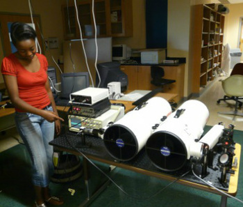
Gisele, a Computer Science major at Spelman, points at the signal on the oscilloscope.
The PEARL research team is comprised primarily of students, with Dr. Peter Chen as the faculty adviser and Haviland Forrister, an Agnes Scott graduate, as a research consultant and part-time employee. The lidar system was built by the students with the advice and aid of Dr. Chen. Originally constructed across two black breadboards, PEARL is a multi-part system containing transmitting optics, a transmitting telescope, a receiving telescope, receiving optics, receiving electronics, and a software system that inputs electronic signals and outputs lidar data.
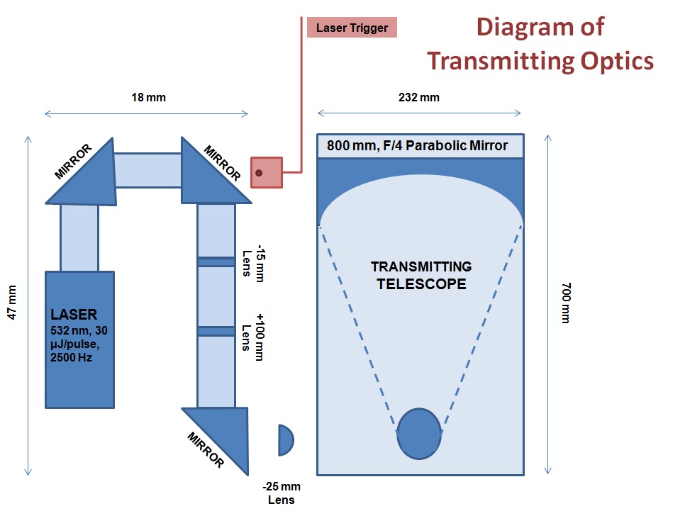
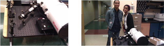
The original transmitting optics can be seen on the far right, on the other side of the telescopes; the diagram of the final transmitting optics is in the diagram below. A laser pulses light onto two mirrors and through two lenses before being focused into the transmitting telescope. Laser light is transmitted out of the transmitting telescope (on the left), is bounced off particles of an object (like, say, molecules in the air or the wood grains on the door), and is received by the receiving telescope (on the right).
The original transmitting optics can be seen on the far right, on the other side of the telescopes; the diagram of the final transmitting optics is in the diagram below. A laser pulses light onto two mirrors and through two lenses before being focused into the transmitting telescope. Laser light is transmitted out of the transmitting telescope (on the left), is bounced off particles of an object (like, say, molecules in the air or the wood grains on the door), and is received by the receiving telescope (on the right).
|
|
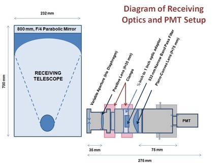
The receiving telescope directs the light toward the receiving optics.
The original receiving optics can be seen in the image at the top, situated
to the left of the telescopes. A diagram of the current receiving
optics is displayed above (right). The photomultiplier tube (PMT) shown at the
end of the receiving optics receives the focused backscattered light and
produces a voltage that corresponds to the number of light counts.
This signal is amplified with a pre-amplifier and then sent to the
computer. The computer software, operated on Labview, inputs the
magnified signal and displays graphs of the amount of light intensity
versus altitude. A second graph displays this intensity versus altitude
as a function of time.
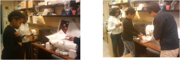
Jessica Robinson and Gisele Izera Munyengabe assist Peter Chen in opening and setting up the first telescope for the system.
Initial setup of the transmitting optics of the lidar system (left). Lidar students Jessica Robinson and Justin Perry pose next to the old transmitting optics (right).
STill a work in progress
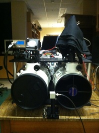
PEARL still has a way to go before we are satisfied. The picture to the right shows the system as it was in August 2012. Since then, we have had many construction and software developments detailed below. From there, we are hoping to miniaturize the system by the end of Summer 2013 so that the lidar is more portable and able to be transported to far locations via car. Currently, the system measures .8 x.62 meters, due to the height of the PMT placement, the size of the breadboards, and the size of the telescopes. We need to obtain and install shorter breadboards and find a way to mount the receiving optics horizontally rather than vertically, possibly with the use of a mirror. Soon, we will receive a third short range telescope and short range PMT to attach to the system, and this PMT will also need to be horizontal. We currently have a surface mirror that we rotate to send the laser light from the telescope upwards into the atmosphere. We use a music stand to hold the mirror in place at a particular angle, but the stand is not stable enough for precise data. We want to construct and build, or otherwise buy, a stable mounting structure for the mirror that allows us to tilt the mirror. Preferably, the structure would have an attachable motor that we can control via Labview to tilt the lidar to a designated angle, rather than estimating the angle with a protractor.
REcent CONSTRUCTION DEVELOPMENTS
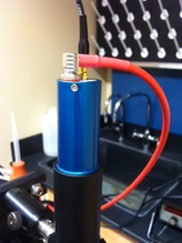
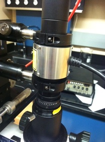
The new PMT.
1) We received and installed the new Photomultiplier Tube (PMT), which translates the incoming light into something that a computer can read in -- current. Our shiny new PMT is shown to the left. Luckily, this one does not have to be covered up by the "witches' hat" that we used to protect the old PMT from excess light. PMTs are notably sensitive to light since they take in light and convert it to current. Too much light harms the PMT and makes it inoperable. Thankfully, this one fit right into the lens tube, so we did not need any other protection on top of it. We can now take the system into whatever lighted environment we wish! However, direct sunlight might not be the best idea...
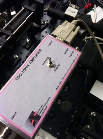
2) We received and installed a new preamplifier. After several studies done between our old preamplifer and the transimpedance amplifier lent to us by Gary Gimmestad, from the Georgia Tech Research Institute, we concluded that a transimpedance amplifier produced higher signal gain, less noise, and no "ringing." Our new amplifier increases the signal we get from the PMT by 100,000 times! It is the pretty pink-and-silver box in the lower left.
3) We received and installed a new filter oven for our narrow bandpass filter. The narrow bandpass filter (centered at 532 nm) is what blocks out all non-532 nm light. This allows us to make sure that we are nearly only seeing the laser light that is reflected back at us, rather than including all of the sunlight at all of its wavelengths, light bouncing off of cars, light from the ceiling fluorescent bulbs, etc. The filter oven keeps the bandpass filter at a constant temperature so as to prevent the set wavelength (532 nm) from changing. We wouldn't want to only be able to see sunlight on a hot day because our filter can no longer see our wavelength!
4) Finally, we most recently received a new Liquid Crystal Variable Retarder (LCVR). This allows us to depolarize our outgoing signal and thus change the "angle" of the outgoing light. Spherical objects like water droplets or most aerosols should reflect all angles of lights. However, non-spherical, "spiky" objects like pollen in the boundary layer or ice particles in high-altitude clouds should only reflect light at a certain angle. Therefore, if we change the angle, we shouldn't be able to seen the pollen or ice! If we send out one angle for a few minutes and then another angle for a few minutes, then we can determine whether the "aerosol" we are seeing in the boundary layer is primarily pollen or some spherical aerosol. There are also set "depolarization ratios" (a ratio of the depolarized/angled signal vs. the original signal) for certain types of particles or aerosols, which means we might be able to determine what category of aerosols we are seeing in the air!
The new transimpedance amplifier.
|
|
RECENT SOFTWARE DEVELOPMENTS
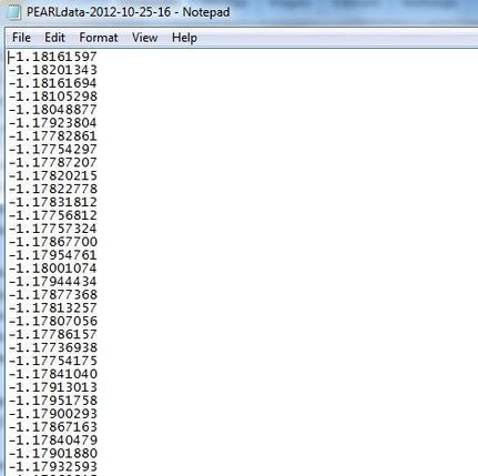
An example of the lidar data outputted from Labview.
Notorious Scott and Gisele Munyengabe programmed the Labview program that runs the lidar system to save the lidar data collected and averaged over a minute as a text file. The text file looks like the picture to the left, where each of the values correspond to a height interval. The first number corresponds to 0 m, the second to 6 m, the third to 12 m, and so on. By plotting this data versus the height interval, correcting for the background light due to sunlight, and correcting for the range at which we receive the signal (farther away signals seem fainter due to their distance, so we multiply the signal by range squared), we can obtain a vertical profile of the atmosphere fora particular minute.
Haviland Forrister recently developed a MATLAB program called ProdPearl that allows us to average several minutes of data together so that we can more clearly see the top of the boundary layer in the vertical profile plot. By averaging the signal we receive back over several minutes, we can cut down the excess noise at higher altitudes. This means that our boundary layer signal also looks a lot clearer, and we can determine the relative aerosol density in that layer.
Haviland also created an Excel spreadsheet that allows us to scale our lidar data to upper air (molecular density of the atmosphere) data and thus determine what is pure aerosols vs. what is normal air (like nitrogen). We then used this spreadsheet to calibrate the PEARL system here at Spelman College to the EARL system (another lidar) over at Agnes Scott College.
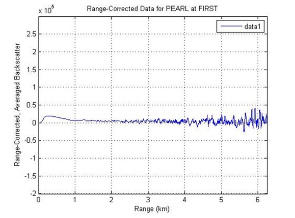
In the graph tbelow, the bump in signal to the left is the "boundary layer," which contains most of the aerosols from car exhaust, pollen, and other urban pollutants. Above the boundary layer is the "free troposphere," where the winds are not blocked by buildings or trees and can thus flow "free." This is where all the weather (clouds, storms, etc) happen. Jenine McCoy gave a presentation on 4/19/2013 on her research about the difference in air quality as perceived from the boundary layer between Spelman and Agnes Scott College.
Haviland Forrister recently developed a MATLAB program called ProdPearl that allows us to average several minutes of data together so that we can more clearly see the top of the boundary layer in the vertical profile plot. By averaging the signal we receive back over several minutes, we can cut down the excess noise at higher altitudes. This means that our boundary layer signal also looks a lot clearer, and we can determine the relative aerosol density in that layer.
Haviland also created an Excel spreadsheet that allows us to scale our lidar data to upper air (molecular density of the atmosphere) data and thus determine what is pure aerosols vs. what is normal air (like nitrogen). We then used this spreadsheet to calibrate the PEARL system here at Spelman College to the EARL system (another lidar) over at Agnes Scott College.
In the graph tbelow, the bump in signal to the left is the "boundary layer," which contains most of the aerosols from car exhaust, pollen, and other urban pollutants. Above the boundary layer is the "free troposphere," where the winds are not blocked by buildings or trees and can thus flow "free." This is where all the weather (clouds, storms, etc) happen. Jenine McCoy gave a presentation on 4/19/2013 on her research about the difference in air quality as perceived from the boundary layer between Spelman and Agnes Scott College.